Excel help please - any wizards on NSC?!

[Goldstone1976]

So your formula in your column H would be =IF(SumProduct(--Isnumber(search(A1,B:F)))>0,INDIRECT("A"&ROW()),"")

Ah, sorry, the table array is in another worksheet so that won't work.

Hmm. I thought Buzzer had it there. Time to call in the expert, I think: [MENTION=451]BensGrandad[/MENTION] , can you help him out please?

 

[clapham_gull]

Its the sort of stuff I get involved in, but not usually with Excel.

I'm not quite sure what you are after but I generaly use something like Jaccard Coefficient in conjuction with K Grams...

..after cleaning the strings.

It's best to work out that data upfront.

I'm on holiday at the mo, but PM me after Easter if it's some sort of fuzzy matching you are after.

The above technique will take a single phrase and compare it's simularity against a number of others.

.. Basically spell checking which is just maths really.

The long list of words is basically a dictionary.

I tend to use SQL more than Excel but it's the same type of technique.

Sent from my LG-K520 using Tapatalk

 

[portlock seagull]

In which case just put my formula in column I as follows:

=IF(H3=TRUE,INDIRECT("A"&ROW())," ")

You Sir, are a genius! Thank you Lord Buzzer, I now need to replace the "A"&ROW(... bit with my table array on another s/s, so it's looking at that value instead. But I think I can do that and hopefully it'll compare the two workbooks and returning said value correctly.

 

[martin tyler]

A beer coming your way at the Wigan game if so!! I'm definitely stuck - and I'm the Excel 'guru' in my business!

Seems Buzzer has beaten me to it.

 

[North East Seagull]

Hi Portlock,
Did you solve this? I was fascinated by your challenge and have come up with another way to do it. It is a two step process but dead easy (has to be - my Excel skills are weak). Will post only if not solved by other posters advice.

 

[father_and_son]

HANDY TIP


VLOOKUP is vastly over-rated given that it takes more CPU and is less flexible that INDEX+MATCH...

So Instead of = VLOOKUP(<SearchCell>,<WholeArray>,<Offset of Search Col>,False)

it is better to be in the habit of using... =INDEX(<ReturnCol>,MATCH(<SearchCell>,<SearchCol>,0)) ...because it uses less CPU time (only makes a difference on VERY large spreadsheets) but the Search Column and Return Column don't even have to be in the same workbook, never mind the same array (so as long as they are the same size)!

 

[m20gull]

Ah, sorry, the table array is in another worksheet so that won't work.

I am not at a PC to check but I think indirect() will work if you replace "A" with "Sheet1!A" assuming the table is on Sheet1.

Edit: should have checked more recent posts

 

[portlock seagull]

[MENTION=5200]Buzzer[/MENTION] [MENTION=13773]Martin[/MENTION]Tyler [MENTION=865]clapham_gull[/MENTION]

Hi again, very grateful for all the support so far but applying the above to my actual data isn't working because I'm on different sheets. I've been banging head against wall a lot this morning!! So decided to present screenshots of exactly how it's laid out so I can copy the formula exactly as it's given.

Sheet 1 is where I'm trying to return in col.I the number of points (shown in Sheet 2, col.A) if the name of the team shown in Col.G of Sheet 1, exists in the table array of different team spellings shown in Sheet 2, col.B to E)

Sheet 1 looks like this:


Sheet 2 looks like this:


In summary, I've found the spelling variation in the Sheet 2's table array, if there's a 'True' value in col.H on Sheet 1. Adjacent to that, I now want it to retrieve the corresponding number of points on sheet 2 if it's found the spelling exists.

My thanks so far, sorry but I've been applying all the help but not quite getting there

 

[portlock seagull]

Seems Buzzer has beaten me to it.

Not quite - still struggling Are you still able to assist, see my post 28

 

[portlock seagull]

In which case just put my formula in column I as follows:

=IF(H3=TRUE,INDIRECT("A"&ROW())," ")

Hi Buzzer, see my post 28 - so sorry, I just couldn't get that to work given the data is on a 2nd sheet. I've laid out as per my actual s/s, are you able to assist still please?

 

[portlock seagull]

Hmm. I thought Buzzer had it there. Time to call in the expert, I think: [MENTION=451]BensGrandad[/MENTION] , can you help him out please?

And thanking you for assisting to!

 

[portlock seagull]

HANDY TIP


VLOOKUP is vastly over-rated given that it takes more CPU and is less flexible that INDEX+MATCH...

So Instead of = VLOOKUP(<SearchCell>,<WholeArray>,<Offset of Search Col>,False)

it is better to be in the habit of using... =INDEX(<ReturnCol>,MATCH(<SearchCell>,<SearchCol>,0)) ...because it uses less CPU time (only makes a difference on VERY large spreadsheets) but the Search Column and Return Column don't even have to be in the same workbook, never mind the same array (so as long as they are the same size)!

Thanks - but how would you apply this to resolve my issue (see post 28)

 

[martin tyler]

Not quite - still struggling Are you still able to assist, see my post 28

I'll have a look today see if I can get it working from what you shown there in28

 

[portlock seagull]

I'll have a look today see if I can get it working from what you shown there in28

Thank you so much! Sorry to put you (all) to so much trouble. It's very much appreciated.

 

[father_and_son]

Thanks - but how would you apply this to resolve my issue (see post 28)

=INDEX('Sheet2'!A:A,MAX(IFERROR(MATCH('Sheet1'!G2,'Sheet2'!B:B,0),0),IFERROR(MATCH('Sheet1'!G2,'Sheet2'!C:C,0),0),IFERROR(MATCH('Sheet1'!G2,'Sheet2'!D,0),0),IFERROR(MATCH('Sheet1'!G2,'Sheet2'!E:E,0),0)))


So:
1. look for G2 ("Brighton&HA") in Column B and if it isn't there return a zero, else return it's row number
2. look for G2 ("Brighton&HA") in Column C and if it isn't there return a zero, else return it's row number
3. look for G2 ("Brighton&HA") in Column D and if it isn't there return a zero, else return it's row number
4. look for G2 ("Brighton&HA") in Column E and if it isn't there return a zero, else return it's row number

5. Take the Maximum value of the above... so, providing what you are looking for is in one of the columns, you find the row number it's in. If it isn't in any of the columns then you will get zero... which gives an error in the final step.

6. Finally, go down Column A to the row determined in step 5 and you will have the points for "Brighton&HA"



[The smiley face is <Colon Capital D>. I know Excel but I don't know how to turn off smiley's in NSC]

 

[Dave the OAP]

I'd be eternally grateful if anyone wants to assist, it's to do with finding name variations within a table array and if found, returns a value from another column within that table array.

Table Array has these variations on a name by column e.g.
(A = 92pts)
B =Brighton
C=Brighton&HA
D=Brighton&HoveAlbion
E=BrightonHoveAlbion
F=BrightonAndHoveAlbion

I'm looking to find Brighton&HoveAlbion (for sake of the following, let's call that A1), so using 'SumProduct(--Isnumber(search(A1,B:F)))>0' it returns 'True' because 'Brighton&HoveAlbion' is indeed one of the spelling variations in column D. So far so good.

However, having found 'A1' within this table array, I also want it to return the value that's in col.A e.g. 92 pts - anyone know how?! Basically I'm searching for variations on a company name within a massive table array and if found, I want to also return the associated value.

Speaking as a ITIL trained Change manager, switch it off and on again

You have been charged £500 an hour for this information

 

[father_and_son]

=INDEX('Sheet2'!A:A,MAX(IFERROR(MATCH('Sheet1'!G2,'Sheet2'!B:B,0),0),IFERROR(MATCH('Sheet1'!G2,'Sheet2'!C:C,0),0),IFERROR(MATCH('Sheet1'!G2,'Sheet2'!D,0),0),IFERROR(MATCH('Sheet1'!G2,'Sheet2'!E:E,0),0)))


So:
1. look for G2 ("Brighton&HA") in Column B and if it isn't there return a zero, else return it's row number
2. look for G2 ("Brighton&HA") in Column C and if it isn't there return a zero, else return it's row number
3. look for G2 ("Brighton&HA") in Column D and if it isn't there return a zero, else return it's row number
4. look for G2 ("Brighton&HA") in Column E and if it isn't there return a zero, else return it's row number

5. Take the Maximum value of the above... so, providing what you are looking for is in one of the columns, you find the row number it's in. If it isn't in any of the columns then you will get zero... which gives an error in the final step.

6. Finally, go down Column A to the row determined in step 5 and you will have the points for "Brighton&HA"



[The smiley face is <Colon Capital D>. I know Excel but I don't know how to turn off smiley's in NSC]

Been thinking.... this only works if you have a manageable number of columns... There is no easy way to do this that I know of if you have an array of company names that is extremely large...

The easiest solution would be to build a simple custom formula to do what you want to do...

Turn on the Developer Tab (in Excel Options)... Double-Click Visual Basic... On the right, where it say "Project - VBAProject", right click, select "Insert" and "Module"

Add the following to the module...


Public Function FindName(ByVal rRange As Range, sText As String) As Long

Dim lCol As Long, lRow As Long

For lCol = 0 To rRange.Columns.Count - 1
lRow = 0
On Error Resume Next
lRow = Excel.WorksheetFunction.Match(sText, Range(Cells(rRange.Row, rRange.Column + lCol), Cells(rRange.Row + rRange.Rows.Count, rRange.Column + lCol)), 0)
On Error GoTo 0
If lRow > 0 Then
FindName = lRow
Exit Function
End If
Next lCol

End Function








You now have a new function available which returns the row number of a value when looking at a very large array.

now your formula would be

=INDEX('Sheet2'!A:A,FindName('Sheet2'!B1:IV65325,'Sheet1'!G2))

 

[portlock seagull]

=INDEX('Sheet2'!A:A,MAX(IFERROR(MATCH('Sheet1'!G2,'Sheet2'!B:B,0),0),IFERROR(MATCH('Sheet1'!G2,'Sheet2'!C:C,0),0),IFERROR(MATCH('Sheet1'!G2,'Sheet2'!D,0),0),IFERROR(MATCH('Sheet1'!G2,'Sheet2'!E:E,0),0)))


So:
1. look for G2 ("Brighton&HA") in Column B and if it isn't there return a zero, else return it's row number
2. look for G2 ("Brighton&HA") in Column C and if it isn't there return a zero, else return it's row number
3. look for G2 ("Brighton&HA") in Column D and if it isn't there return a zero, else return it's row number
4. look for G2 ("Brighton&HA") in Column E and if it isn't there return a zero, else return it's row number

5. Take the Maximum value of the above... so, providing what you are looking for is in one of the columns, you find the row number it's in. If it isn't in any of the columns then you will get zero... which gives an error in the final step.

6. Finally, go down Column A to the row determined in step 5 and you will have the points for "Brighton&HA"



[The smiley face is <Colon Capital D>. I know Excel but I don't know how to turn off smiley's in NSC]

Hi and thank you, what a bit of code you've written!!

Good news - it worked correctly! But only up to a point, so I'll come clean and present the real data so you can see exactly what I'm talking about (I tried to make it 'footy like' but probably best I just show the RAW data.

Sheet 1:


Sheet 2:


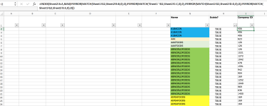
Applying your algorithm, you'll see it returned the correct Company ID (from sheet 2) for the first 3 rows in Sheet 1 i.e. A1Bacon = 406 in sheet 2 and it's returned '406' into Sheet 1 (cells I2,I3&I4)

However, when you move onto the next company - called AAK - in Sheet 1(cell G5), the ID being returned from Sheet 2 is 623 - when it should be 126 (see cell A8). Similarly, AAKFoods (same company, different spelling) I also need to return 126 as the company ID - and it does! However, when move into the next company - called ABWorldFoods - it returns multiple Company IDs (the correct one should be 478, if you look at Sheet2)

Now I've explained properly using the real data, is this something you can resolve please? Or is there even a new way of doing things.

The basic outline of my problem is that dozens of different businesses use the same suppliers but all have different spellings and variations (use or not of punctuation, initials, suffixes, abbreviations etc) which makes comparisons to see if we're already connected to them v.tricky. Hence why we've a table array with multiple spelling variations in Sheet2 to compare Sheet1 against (and return 'true' if it does exist in Sheet2). I just need it to also return the correct Company ID number alongside.

 

[portlock seagull]

Been thinking.... this only works if you have a manageable number of columns... There is no easy way to do this that I know of if you have an array of company names that is extremely large...

The easiest solution would be to build a simple custom formula to do what you want to do...

Turn on the Developer Tab (in Excel Options)... Double-Click Visual Basic... On the right, where it say "Project - VBAProject", right click, select "Insert" and "Module"

Add the following to the module...


Public Function FindName(ByVal rRange As Range, sText As String) As Long

Dim lCol As Long, lRow As Long

For lCol = 0 To rRange.Columns.Count - 1
lRow = 0
On Error Resume Next
lRow = Excel.WorksheetFunction.Match(sText, Range(Cells(rRange.Row, rRange.Column + lCol), Cells(rRange.Row + rRange.Rows.Count, rRange.Column + lCol)), 0)
On Error GoTo 0
If lRow > 0 Then
FindName = lRow
Exit Function
End If
Next lCol

End Function








You now have a new function available which returns the row number of a value when looking at a very large array.

now your formula would be

=INDEX('Sheet2'!A:A,FindName('Sheet2'!B1:IV65325,'Sheet1'!G2))

Hi, I've tried but error message keeps coming back. Developer and Macros is an area I'm really not familiar with though (and it's slightly different set up on a Mac). I read this only after my post 38 mind.

 

[portlock seagull]

I'll have a look today see if I can get it working from what you shown there in28

See 38 for the actual raw data (assuming you're able to help still) - have to say, this is a bit of a bugger. Fuzzy logic and some!